
Current Sensing Architectures in High-Speed GaN Servo Drives: In-Line Phase Current vs Low-Side Shunts vs Coreless Magnetic Sensors
Compare current sensing in GaN servo drives: low-side shunts, in-line shunts and magnetic sensors. Use timing and thermal examples plus an RFQ checklist to select.
Current sensing in GaN servo drives determines when phase-current feedback is valid, how much heat the measurement path adds, and which fault currents the drive can detect. Higher PWM frequency can reduce current ripple in a low-inductance motor, but leaves less time for analog settling, ADC acquisition and control computation. GaN switching alone does not establish current-loop accuracy or bandwidth.
This guide compares low-side three-shunt sensing, in-line phase shunts, and coreless magnetic sensors for engineering and procurement teams selecting low-voltage robot-joint and AMR drives. A single DC-link shunt is included as a cost-oriented reference.
Selection summary:
- Choose low-side shunts when the supplier demonstrates valid sampling windows throughout your required speed, load and modulation range.
- Consider in-line sensing when low-side sampling windows restrict operation. The phase path remains observable through both switch states, but switching edges still require settling or filtering.
- Compare magnetic sensors with the actual shunt resistance and package conductor resistance. Magnetic sensing does not automatically mean lower loss.
- Qualify the complete fault-detection and gate-disable path separately from the FOC feedback channel. Neither topology nor sensor isolation establishes Safe Torque Off (STO) capability.
Reviewed: October 29, 2026. Scope: Global, English-language engineering selection guide. The focus is nominal 24V–60V DC PMSM/BLDC servo drives, with higher buses discussed only where component ratings permit. Battery charging, regeneration and switching overshoot must fit the actual drive and sensing limits. The 50–200 kHz PWM examples are analysis scenarios, not advertised operating ranges for every component or product linked here.
Method and limitations: The timing and loss examples below are reproducible calculations using stated assumptions, not measurements of a GaN Servo Drives product. Component specifications come from the primary sources linked beside the claims and listed at the end. No bench validation, customer case study, universal ambient rating or safety certification is asserted. Confirm the exact part suffix, datasheet revision and installed thermal conditions before design approval.
For a product discussion, start with the GaN low-voltage servo drive range and ask for the sensing topology and validation data for the specific hardware revision.
1. Why High-Frequency GaN Switching Challenges Current Sensing
1.1 Slew Rate and Capacitive Displacement Current
A phase-node voltage step can couple into the analog front-end through parasitic capacitance. The displacement-current estimate is I = C × dV/dt. For an illustrative 5 pF capacitance and 50 V/ns edge:
I = 5 × 10⁻¹² F × 50 × 10⁹ V/s = 0.25 A.
This is an instantaneous coupling estimate, not the current guaranteed to enter an amplifier input. Its return path, input protection and layout determine the resulting error. Measure output disturbance and recovery at the actual bus voltage, edge rate, load current and temperature; a DC common-mode rejection specification cannot establish switching-edge performance.
1.2 PWM Period and Control Delay
At 100 kHz, T_PWM = 1/f_PWM = 10 µs; at 200 kHz it is 5 µs. The sampling trigger, analog settling, conversion or digital-filter delay, computation and PWM update must fit the chosen control schedule.
Sensor bandwidth is not closed-loop current bandwidth. For a pure delay, the additional phase lag is 360° × f_loop × t_delay: 2 µs adds 3.6° at 5 kHz. Analog poles, digital filters and PWM timing add further lag. Ask for the measured loop response rather than inferring it from switching frequency.
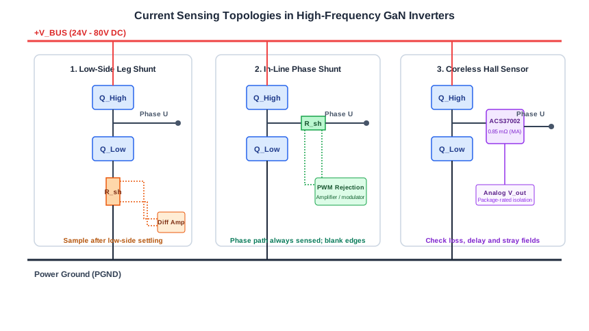
2. Architecture Comparison: Circuit Topologies
In-line describes where current is sensed; shunt or magnetic describes how. An in-line shunt can feed a ground-referenced amplifier with sufficient common-mode range, or a floating isolated conversion stage. These implementations have different supply, isolation and latency requirements.
3. Architecture 1: Low-Side Three-Shunt Sensing
3.1 Operating Principle and Cost Appeal
A resistor in each low-side leg measures current near power ground. This usually reduces the required amplifier common-mode range and can allow MCU-integrated amplifiers. It does not remove ground bounce or the need for bidirectional input and transient checks. GaN reverse conduction is device- and gate-bias-dependent; it should not be modeled as a fixed silicon body-diode drop.
3.2 Minimum Valid Sampling Window
A low-side leg shunt provides usable phase-current information during suitable conduction states, after edge disturbances have settled. Reverse conduction can also carry shunt current; the switch being commanded on is not the only possible current path.
For a conservative timing budget, assume sequential intervals:
t_min = t_dead + t_blanking + t_settle + t_acquisition
An illustrative budget is 40 ns + 150 ns + 250 ns + 200 ns = 640 ns. These are assumed design inputs, not guaranteed component limits. Some intervals may overlap in a real implementation. ADC conversion and computation must also finish before the control update deadline, even if they occur after the sampling aperture.
3.3 Worked Example: Duty Ratio Is Not Modulation Index
For one contiguous low-side interval, the simplified relation is t_low = (1 − D) × T_PWM, where D is that leg's high-side duty ratio:
| PWM frequency | High-side duty D | Available low-side interval | Against assumed 640 ns budget |
|---|---|---|---|
| 16 kHz | 90% | 6.25 µs | Above budget |
| 16 kHz | 95% | 3.125 µs | Above budget |
| 100 kHz | 90% | 1.0 µs | Above budget |
| 100 kHz | 95% | 0.5 µs | Below budget |
| 200 kHz | 85% | 0.75 µs | Above budget |
| 200 kHz | 90% | 0.5 µs | Below budget |
For this simplified model, D_max = 1 − t_min/T_PWM: 93.6% at 100 kHz and 87.2% at 200 kHz. These are per-leg duty bounds under the stated assumptions, not universal SVPWM modulation limits. Center-aligned pulse splitting, vector sector, ADC channel sequencing and the availability of two independent phase measurements change the usable windows.
Pulse shifting or reconstruction can extend the operating range. Require the supplier to show its effect on voltage distortion, current error and torque ripple across the required operating envelope. Low-side sensing is acceptable when those results meet the application requirements.
3.4 Ground Bounce and Layout
The relation V = L × di/dt explains why Kelvin shunt connections and controlled return paths matter. As a sensitivity example, 2 nH at 5 A/ns gives 10 V across that inductance. This is not a prediction of gate-source voltage: the actual coupling depends on the power loop, driver return and package. Validate the layout with switching waveforms rather than treating topology alone as a failure verdict.
4. Architecture 2: In-Line Phase Shunt Sensing
4.1 Phase Visibility and Its Limits
A phase shunt stays in series with the motor winding through high-side and low-side conduction. It removes the requirement to wait for low-side conduction, which can help at high duty ratios. It does not make every sample valid: avoid unsettled edges and account for analog or digital-filter delay. Bootstrap supply requirements, dead time and the control strategy can still limit achievable duty ratio.
In-line sensing can observe some phase-to-chassis fault currents that bypass low-side resistors. Coverage depends on fault location, grounding and return path. Detecting a fault does not guarantee sufficiently fast gate turn-off, and ordinary overcurrent shutdown does not establish a validated STO function.
4.2 Common-Mode Range and Transient Recovery
At 20 A, a 1 mΩ shunt produces only 20 mV while its common-mode voltage follows the switching node. Select the front-end for negative excursions, maximum charged bus voltage and overshoot, then verify output recovery at the intended ADC trigger. Isolation working voltage, transient immunity and static CMRR are different specifications.
4.3 Enhanced PWM-Rejection Amplifiers: INA241 Example
TI specifies the INA241A for a −5 V to +110 V operating common-mode range, enhanced PWM rejection and switching frequencies up to 125 kHz. Its listed step-response settling time to 1% is 1 µs. That settling figure does not describe a fixed internal output-hold interval or guarantee the complete channel's recovery under every switching transient.
Check the selected gain, output swing, ADC reference and filter loading. A 200 kHz analysis example in this guide is outside that stated PWM frequency support; choose and validate a suitable front-end instead of extrapolating the INA241 specification.
4.4 Isolated Delta-Sigma Modulators: AMC1306 Example
The TI AMC1306M25 provides a reinforced isolation barrier and an uncoded bitstream; Manchester encoding is available on other family variants. TI lists 50 kV/µs minimum CMTI and 100 kV/µs typical. Compare the guaranteed value with measured switching edges, including design margin.
The floating measurement side needs an appropriate supply. A digital filter in a compatible MCU or FPGA converts the bitstream into current samples. Filter order, clock rate and oversampling ratio set the resolution and delay trade-off; isolation does not make the signal immune to all noise. Verify the exact MCU peripheral rather than assuming every device in a family includes a suitable filter.
4.5 Worked Thermal Example for Phase Shunts
Assume 60 A RMS per motor phase, three equal 1.5 mΩ in-line shunts, and constant resistance for this first estimate:
P_phase = I_phase,RMS² × R = 60² × 0.0015 = 5.4 W
P_three_phases = 3 × 5.4 = 16.2 W.
This is not DC bus current, peak phase current or a demonstrated continuous product rating. A lower-resistance shunt reduces loss but also reduces signal amplitude and tightens offset/noise requirements. Include hot resistance, resistor derating and the installed thermal path before approving the design.
5. Architecture 3: Coreless Magnetic Sensors
5.1 Operating Principle and Isolation
A coreless Hall sensor measures the magnetic field generated by its primary conductor. The ACS37002 datasheet describes differential Hall sensing and package-dependent isolation. ACS37002 is a Hall device; it is not a TMR sensor. Other magnetic technologies require their own qualification.
Isolation is finite. Check the exact package's working voltage, withstand test rating, creepage and clearance; a kilovolt withstand test does not mean unlimited continuous common-mode voltage.
5.2 Package-Specific Loss Comparison
The cited ACS37002 Rev. 11 datasheet lists 0.85 mΩ for MA and 1 mΩ for LA. Allegro's product page also advertises an MC package down to 0.27 mΩ. These values belong to different packages; obtain the matching datasheet and orderable suffix before comparing them.
Using the 0.85 mΩ MA value with the same illustrative 60 A RMS phase current:
P_phase = 60² × 0.00085 = 3.06 W; three phases total 9.18 W.
That is about 43% less conductor loss than the 16.2 W shunt example. Conversely, three 0.5 mΩ shunts would dissipate 5.4 W under the same assumptions, less than this magnetic package. These calculations exclude IC supply power and PCB losses, and do not qualify any package for continuous 60 A operation. Check its thermal limits and peak measurement range separately.
5.3 Bandwidth and Protection Delay
The ACS37002 Rev. 11 datasheet lists 400 kHz bandwidth, 1.1 µs typical signal response and 1 µs typical overcurrent response. The product page lists a 1.5 µs maximum overcurrent response. Use the applicable suffix's guaranteed limits when designing protection; neither value supports a claim of sub-300 ns fault shutdown.
A control-feedback channel may be too slow for a particular GaN short circuit. Qualify a dedicated protection path where needed, including threshold crossing, blanking, comparator delay, logic, gate-driver delay and device turn-off. The allowable total time comes from the selected power stage's fault withstand capability.
5.4 Stray Fields in Compact Robot Joints
Differential Hall sensing reduces sensitivity to uniform external fields, but motor/brake field gradients and nearby conductors can still create errors. Test zero-current offset and loaded gain with the rotor swept through its positions, the brake energized and released, and neighboring phases carrying current.
There is no universal 10 mm clearance or shielding recipe. Grounded copper is not an effective general shield for static magnetic fields. Select spacing, orientation and any magnetic shielding from measured field susceptibility, checking saturation and assembly tolerances.
6. Reference Architecture: Single DC-Link Shunt
A single DC-link shunt reduces channel count. Phase-current reconstruction requires samples in identifiable active switching states, so short or coincident vector intervals can require pulse modification or an observer. At high PWM frequency this is a demanding timing problem, not an automatic application ban.
For precision robotics, accept this option only with evidence of current reconstruction accuracy, torque ripple and control stability across startup, low speed, high modulation and regeneration. A lower BOM cost alone does not resolve missing sampling windows.
7. Architecture Selection Matrix
This matrix is a screening aid, not a set of guaranteed frequency, cost or safety ratings. The thermal row uses 60 A RMS phase current and the resistances stated above. Low-side resistor heating must instead use the RMS current actually flowing through each leg shunt over its switching states.
| Evaluation metric | Low-side three-shunt | In-line shunt + amplifier | In-line shunt + isolated modulator | Coreless Hall sensor | Single DC-link shunt |
|---|---|---|---|---|---|
| Sensing location | Low-side legs | Motor phase conductors | Motor phase conductors | Motor phase conductors | DC-link return |
| Valid sampling | Suitable settled low-side states | Avoid unsettled switching edges | Include filter response and delay | Include sensor response and settling | Identifiable active-vector states |
| High-duty constraint | Available leg windows | No low-side window constraint | No low-side window constraint | No low-side window constraint | Reconstruction windows |
| Frequency qualification | Derive from timing budget | INA241 lists up to 125 kHz | Check bitstream/filter schedule | Check response and loop margin | Check two-sample reconstruction |
| Main electrical stress | Ground bounce, negative inputs | Full phase common-mode swing | Isolation CMTI and floating supply | Package isolation and transients | Pulsed bus-return current |
| Resistive-loss basis | Leg-shunt RMS waveform | 16.2 W total at 1.5 mΩ/phase | 16.2 W total at 1.5 mΩ/phase | 9.18 W total at 0.85 mΩ/phase | DC-link shunt RMS waveform |
| Fault coverage | Depends on return path | Depends on fault location and shutdown path | Includes filter/protection-path delay | Includes fault-output and shutdown delay | Depends on return path |
| Magnetic susceptibility | Check layout coupling | Check layout coupling | Check layout coupling | Check external field gradients | Check layout coupling |
| Cost drivers | Shunts, channels, calibration | Shunts and PWM-capable amplifiers | Modulators, supplies and filters | Exact package, range and channel count | Reconstruction firmware and validation |
| Evidence to request | Window map and reconstruction error | Common-mode recovery at ADC trigger | Guaranteed CMTI and filter latency | Thermal and stray-field error results | Current error across vector sectors |
For a compact joint program, use these evidence requirements alongside the mechanical constraints on the robot joint servo drive page.
8. Sourcing Strategy and RFQ Checklist
Compare quotations against one shared operating envelope. Include the following in the RFQ:
- Topology and revision: Identify sensor count, part numbers, shunt values, PCB revision and calibration method.
- Operating envelope: State nominal/maximum DC bus voltage, phase RMS and peak currents, peak duration, motor inductance, electrical speed and regeneration conditions.
- Sampling evidence: Request PWM frequency, ADC trigger positions, minimum valid windows, blanking/settling budget and reconstruction behavior at the required modulation range.
- Transient immunity: Request waveforms at the actual maximum common-mode voltage and slew rate, with measurement setup, temperature and error acceptance limit.
- Thermal and accuracy budget: Include shunt/conductor hot resistance, sensor offset, gain, ADC/reference error, filtering and calibration residuals across the required ambient range.
- Magnetic susceptibility: For magnetic sensors, request error with the installed motor, brake and neighboring conductors in their worst operating states.
- Fault shutdown: Require a documented fault-current path and worst-case end-to-end turn-off time against the power-stage limit. Request STO evidence separately if the machine requires that function.
- Control performance: Specify required loop bandwidth, stability margin and acceptable torque ripple; request measured results at representative load and speed points.
- Supply continuity: Confirm exact orderable suffixes, lifecycle and lead times. Treat an alternate sensor as an engineering change requiring pinout, gain, timing and thermal requalification.
9. Frequently Asked Questions
Can low-side shunts work at 100 kHz?
Yes, if valid sampling windows and the complete control schedule meet the requirements. The 640 ns example shows why high per-leg duty ratios become difficult; it does not prove that all low-side drives fail above a fixed modulation index. Ask for a window map and measured current error across the operating envelope.
Does in-line sensing guarantee 100% duty cycle?
No. It removes the low-side-conduction requirement for observing phase current, but transient settling, gate-drive supply constraints, PWM strategy and protection still apply. Qualify the achievable output voltage and current feedback together.
Does a magnetic sensor always run cooler than a shunt?
No. Compare actual hot conductor resistances and sensor supply power. In the worked example, 0.85 mΩ produces less loss than 1.5 mΩ but more than 0.5 mΩ. Package current range, cooling and board copper determine whether the calculated loss is acceptable.
How can current-sensing error affect joint noise?
Offsets, phase gain mismatch and switching artifacts can enter the FOC regulator and create torque disturbances. Motor electromagnetic forces, mechanics and controller tuning also contribute to sound and vibration. Measure current error, torque ripple and acoustic response together before assigning the cause to the sensor.
What is the trade-off between an analog amplifier and an isolated modulator?
An analog amplifier connects to an ADC and needs a compatible input/output range and sampling schedule. An isolated modulator adds a floating supply and digital filtering; its resolution and delay depend on configuration. Compare total channel latency and guaranteed transient performance rather than assuming either implementation is universally faster or safer.
How should temperature drift be compared?
For a shunt, relative resistance change ≈ TCR × temperature change. At 50 ppm/°C over 80°C, the contribution is 0.4%, before amplifier and ADC errors. For a magnetic sensor, include offset, sensitivity, noise and calibration residuals across temperature. A sensitivity-error specification alone is not the total current error, especially near zero current.
10. Next Steps for Engineering and Procurement
Select the architecture that demonstrates valid samples, acceptable installed loss and a qualified protection path over your motor's operating envelope. Low-side sensing can be economical; in-line shunts can simplify current visibility; magnetic sensors can provide isolation and package integration. Each still needs application-specific validation.
For battery-powered traction, review the AMR and mobile robot servo drive application. For joint integration or a custom form factor, use the OEM engineering discussion to share your bus voltage, phase RMS/peak current, PWM target, motor inductance and enclosure cooling conditions. Request a revision-specific sensing and validation plan before committing to samples or volume supply.
Sources and References
The following manufacturer documents support the component examples. They do not validate a complete servo drive or the illustrative calculations above. Checked October 29, 2026.
- Texas Instruments — INA241A product specifications and linked datasheet: operating common-mode range, enhanced PWM rejection, supported switching frequency and step-response settling.
- Texas Instruments — AMC1306M25 product specifications and linked datasheet: isolated bitstream conversion, CMTI ratings and digital-filter requirements.
- Allegro MicroSystems — ACS37002 datasheet, Rev. 11, August 14, 2025: pages 1–2 identify Hall sensing, MA/LA conductor resistances, response times and package-dependent ratings.
- Allegro MicroSystems — ACS37002 product page: additional MC-package resistance and maximum overcurrent-response information. Obtain the matching package documentation before applying those values.
Author

More Posts
Evaluating Monolithic 3-Phase GaN Servo Micromodules: 2026 Procurement & Engineering Guide
A 2026 engineering and procurement guide to monolithic 3-phase GaN servo micromodules, thermal limits, supplier risk, sourcing checklist, and fit for compact robotics.

Sourcing Decentralized IP67 GaN Servo Drives: Wiring Cost Reduction and Thermal Trade-offs
Global sourcing guide for decentralized IP67 GaN servo drives, covering wiring cost models, thermal derating limits, RFQ evidence, and OEM sourcing CTAs.
How to Specify 48V GaN Servo Drives for Low-Inductance Motors: Eliminating Chokes and Current Ripple
Specify 48V GaN servo drives for low-inductance robotics motors: current ripple limits, choke elimination, EMI risks, RFQ checks, and sourcing trade-offs.